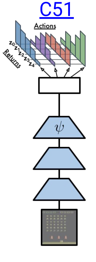
C51 is one of my favourite RL algorithms, because of its unique approach of calculating the distribution of returns rather than calculating the expectation of rewards. I firstly heard of this approach in this(AI Prism: Deep RL Bootcamp) youtube video. Someone with basic knowledge of DQN and policy gradient algorithms should watch the complete course. C51 has some modified versions too like QR-DQN and IQN. C51 can be easily visualised compared to QR-DQN and IQN, so before going into them, we must know about C51 and the distributional perspective of RL. I have implemented C51 and QR-DQN, and this blog will help readers to understand Distributional RL. I have also written some of my observations. You can find my code here.

Distributional RL

The idea behind learning the distribution of future returns instead of just learning the expected value is to make the model capable of learning intrinsic randomness(Stochastic dynamics, Stochastic reward) of the returns. Consider a person who bought a lottery ticket and so did 1000 other people. 10 lucky people will get 1M dollar if they win, which is 1 in a 100 chance he will get 1M dollars otherwise he will get 0 dollars with chance 90 in 100 so, expected amount a person will get is 1000 dollars and traditional value-based Deep RL algorithms learn to calculate the expected reward, but in reality he will never get reward of 1000 dollars, i.e. we are getting false knowledge of the possible returns. Returns can be multimodal like in the lottery scenario due to which variance is too high which makes the convergence difficult.

Distributional Bellman Equation

Very similar to the Bellman Equation, the \(Distributional\) \(Bellman\) \(Equation\) is expressed as:
\(Z(s,a) = r + \gamma Z(s^\prime,a^\prime)\)
Where \(Z\) represents the distribution of future rewards, unlike \(Q\) which is a scalar. According to the paper, the \(distributional\) \(Bellman\) \(equation\) states that the distribution of \(Z\) is characterized by the interaction of three random variables: the reward \(R\), the next state-action\((X^\prime,A^\prime)\), and its random return \(Z(X^\prime,A^\prime)\). By analogy with the well-known case, we call this quantity the \(value\) \(distribution\).

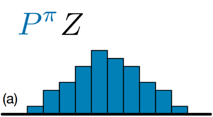
Value distribution

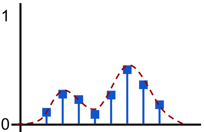
The output of the C51 algorithm is Discrete Probability Distribution of returns as shown above. Discrete distribution can easily take the form of multimodal distribution. The vertical axis represents the probability. The horizontal bars are called atoms, and they are the “canonical returns” of the distribution. Atoms are placed at regular intervals on the \(return\) \(axis\), which ranges from minimum possible return to maximum possible return.

Distributional Bellman equation dynamics

Next state distribution under policy \(\pi\): \(Z(s^\prime,a^\prime)\) where \(s^\prime\) and \(a^\prime\) are next state obtained after transition from state \(s\) taking action \(a\) and \(a^\prime\) is action taken at state \(s^\prime\).

Multiply each support(distribution) by the discount factor \(\gamma\), since \(\gamma\) is less than 1 it shrinks the whole distribution towards 0.

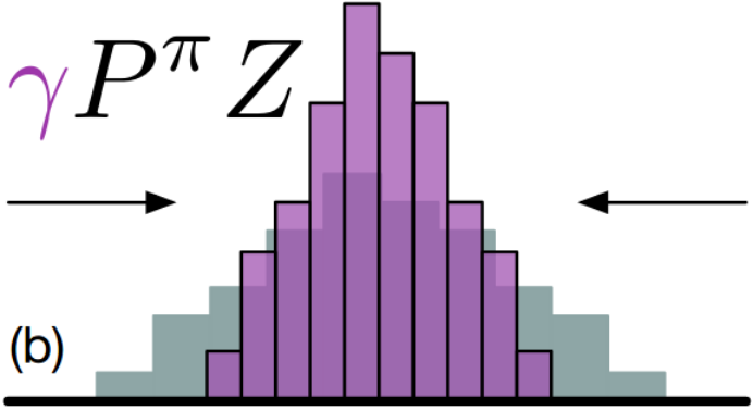
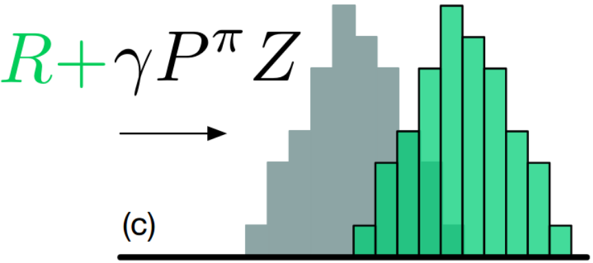
Adding reward \(r\) to each support(distribution), which causes a shift in the distribution.

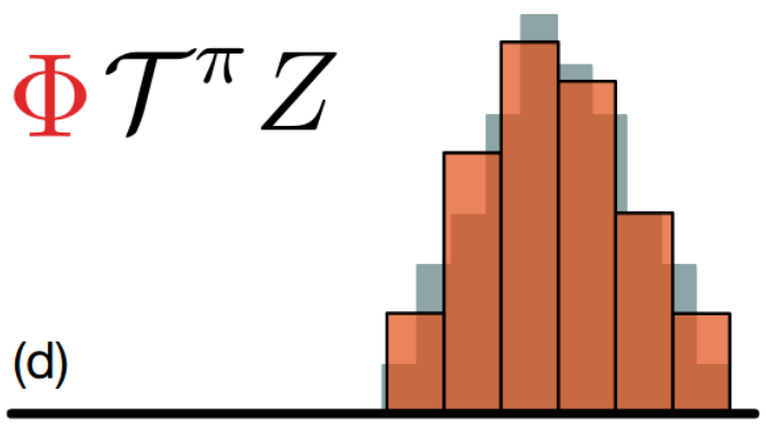
All the above operations has changed the atoms, so we need to change the support of the target distribution with the original support, i.e. projection.

Loss Function

The paper uses Cross Entropy(Kullback–Leibler divergence) loss function:
\(loss\) \(=\) \(-\sum_{i=1}^Ny_{i}\log(p_{i})\)

\(N\) - Number of atoms
\(log\) - the natural log
\(y_{i}\) - target for \(i\)th atom
\(p_{i}\) - predicted for \(i\)th atom

Earth mover distance

The paper talks a lot about Wasserstein distance, but in practice, they used a KL-based procedure. I tried of on my own to get some results using EDM(Earth movers distance/1st Wasserstein distance) as the loss function, but it is not stable. I tried different learning-rates and optimizers(SGD, Adam, rmsprop). I got the best result with rmsprop(lr=0.001). You can look for it in my GitHub repository Quest-RL. In the next iteration of the C51 algorithm, i.e. Quantile Regression-DQN, the paper also talks about how we can use Wasserstein distance in practice. I have implemented QR-DQN which you can find here . I will write a blog for the same very soon.

Reference

• Bellemare, Marc G., Will Dabney, and Rémi Munos. 2017. “A Distributional Perspective on Reinforcement Learning.” CoRR abs/1707.06887. http://arxiv.org/abs/1707.06887.
  
• Distributional RL sildes